Optimal design with LOQ data in PopED
Optimization with a model for warfarin
Andrew Hooker
Source:vignettes/articles/handling_LOQ.Rmd
handling_LOQ.RmdDefine a model
Here we define, as an example, a one-compartment pharmacokinetic model with linear absorption (analytic solution) in PopED (Nyberg et al. 2012).
library(PopED)
packageVersion("PopED")
#> [1] '0.7.0'
ff <- function(model_switch,xt,parameters,poped.db){
  with(as.list(parameters),{
    y=xt
    y=(DOSE*KA/(V*(KA-CL/V)))*(exp(-CL/V*xt)-exp(-KA*xt))
    return(list(y=y,poped.db=poped.db))
  })}
Next we define the parameters of this function. DOSEis
defined as a covariate (in vector a) so that we can
optimize the value later.
sfg <- function(x,a,bpop,b,bocc){
  parameters=c( CL=bpop[1]*exp(b[1]),
                V=bpop[2]*exp(b[2]),
                KA=bpop[3]*exp(b[3]),
                DOSE=a[1])
}
We will use an additive and proportional residual unexplained
variability (RUV) model, predefined in PopED as the function
feps.add.prop.
Define an initial design and design space
Now we define the model parameter values, the initial design and design space for optimization. We define model parameters similar to the Warfarin example from the software comparison in Nyberg et al. (2015) and an arbitrary design of one group of 32 individuals.
Simulation
First it may make sense to check the model and design to make sure we get what we expect when simulating data. Here we plot the model typical value and a 95% prediction interval (PI) for the intial design:
plot_model_prediction(poped_db, model_num_points = 500,facet_scales = "free",PI=T)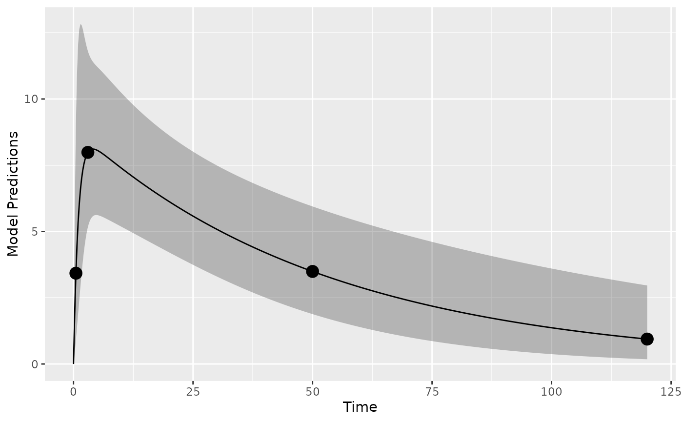
Design evaluation
Next, we evaluate the initial design.
eval_full <- evaluate_design(poped_db)
round(eval_full$rse)| RSE | |
|---|---|
| CL | 5 |
| V | 4 |
| KA | 15 |
| d_CL | 34 |
| d_V | 70 |
| d_KA | 28 |
| sig_prop | 89 |
| sig_add | 36 |
We see that the relative standard error of the parameters (in
percent) are relatively well estimated with this initial design except
for the between subject variability parameter for volume of distribution
(d_V) and the proportional RUV parameter
(sig_prop).
LOQ handling
We assume that the LOQ level is at 2 concentration units. Here shown as a red dotted line.
library(ggplot2)
plot_model_prediction(poped_db, model_num_points = 500,facet_scales = "free",PI=T) +
  geom_hline(yintercept = 2,color="red",linetype="dotted",linewidth=1)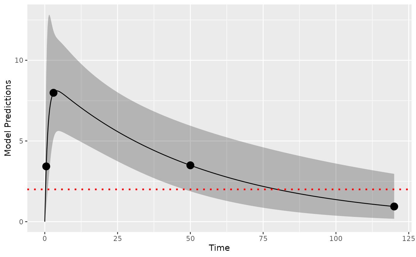
To evaluate the designs we use the design evaluation criteria based
on the “integration and FIM scaling” method (loq_method=1
which is the default) and the “omit observations where PRED<LOQ”
method (loq_method=2) from Vong et
al. (2012) (referred to as the D6 and
D2 methods, respectively, in the presentation by Vong et al.). In the D6
method we:
Enumerate all permutations of each sample point being quantifiable or not (below the lower LOQ, or above the upper LOQ). If sample points have an expected prediction interval (default is 95%,
loq_PI_conf_level = 0.95) that does not overlap the LOQ then the design point is assumed to either always be observed or to always be outside the limit of quantification.Compute the probability of each permutation occurring, filtering out potential realized designs with very low probabilities (default is
loq_prob_limit = 0.001).Evalaute the Fisher Information Matrix (FIM) for all remaining design permutations, assuming no information from any design point if, for that permutation, it is not in within the limits of quantification.
Take the weighted sum of the resulting information matrices.
The D2 method is a simplification of this process where all samples with a typical value prediction (PRED) below the lower LOQ or above upper LOQ are removed from the design before calculating the FIM.
Here we evaluate the initial design with both methods and test the speed of the computations. We see that D6 is significantly slower than D2 (but D6 should be a more accurate representation of the RSE expected using M3 estimation methods).
set.seed(1234)
e_time_D6 <- system.time(
  eval_D6 <- evaluate_design(poped_db,loq=2)
)

e_time_D2 <- system.time(
  eval_D2 <- evaluate_design(poped_db,loq=2, loq_method=2)
)

cat("D6 evaluation time: ",e_time_D6[1],"seconds \n" )
cat("D2 evaluation time: ",e_time_D2[1],"deconds \n" )
#> D6 evaluation time:  0.041 seconds
#> D2 evaluation time:  0.007 deconds
The D2 method is the same as removing the last design point, as you can se below.
poped_db_2 <- create.poped.database(
    ff_fun=ff,
    fg_fun=sfg,
    fError_fun=feps.add.prop,
    bpop=c(CL=0.15, V=8, KA=1.0),
    d=c(CL=0.07, V=0.02, KA=0.6),
    sigma=c(prop=0.01,add=0.25),
    groupsize=32,
    xt=c( 0.5,3,50),
    discrete_xt = list(c(0.5,1:120)),
    minxt=0,
    maxxt=120,
    a=70,
    mina=0,
    maxa=100)
eval_red <- evaluate_design(poped_db_2)
testthat::expect_equal(eval_red$ofv,eval_D2$ofv)
testthat::expect_equal(eval_red$rse,eval_D2$rse)
The predicted parameter uncertainty for the three methods is shown in the table below (as relative standard error, RSE, in percent). We see that the uncertainty is generally higher with the LOQ evaluations (as expected). We also see that the predictions of uncertainty are significantly larger than the D6 method. This too is expected, because the D2 method ignores design points where the model PRED is below LOQ (the last observation in the design), whereas it appears from the previous figure that ~25% of the observations from the last design point will be above LOQ. The M6 method accounts for this probability that the last design point will have data above LOQ and is thus a more realistic assessment of the expected parameter uncertainty.
| Parameter | No LOQ | D6 | D2 |
|---|---|---|---|
| CL | 5 | 6 | 6 |
| V | 4 | 4 | 4 |
| KA | 15 | 17 | 15 |
| d_CL | 34 | 50 | 498 |
| d_V | 70 | 109 | 428 |
| d_KA | 28 | 33 | 113 |
| sig_prop | 89 | 161 | 1444 |
| sig_add | 36 | 118 | 2127 |
ULOQ handling
If needed we can also handle upper limits of quantification. Lets assume we have an ULOQ at 7 units in addition to the LLOQ of 2 units:
library(ggplot2)
plot_model_prediction(poped_db, model_num_points = 500,facet_scales = "free",
                      PI=T, PI_alpha = 0.1) +
  geom_hline(yintercept = 2,color="red",linetype="dotted",linewidth=1) +
  geom_hline(yintercept = 7,color="blue",linetype="dotted",linewidth=1)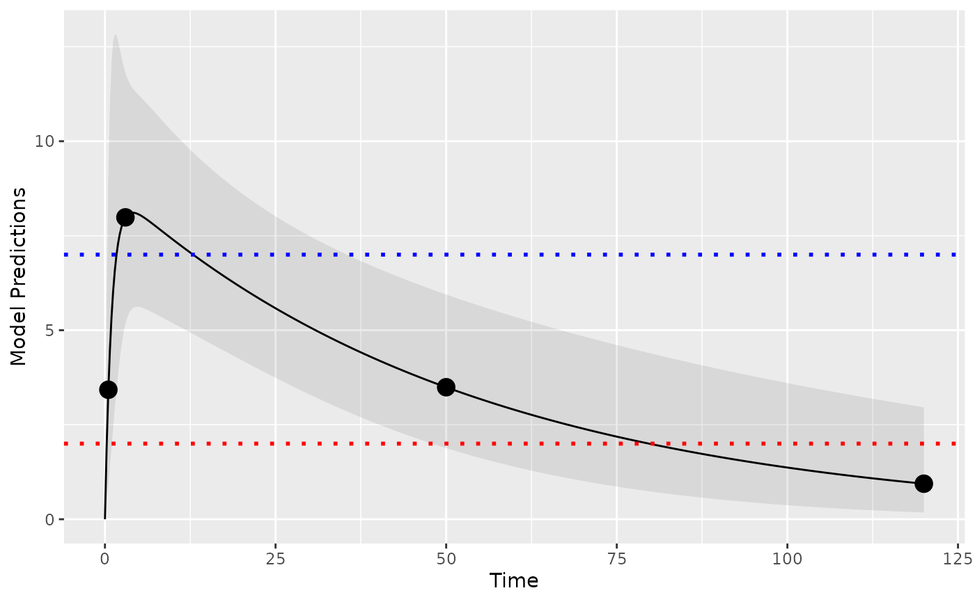
We can then evaluate the design based on the D2 and D6 methods.
eval_ul_D6 <-evaluate_design(poped_db,
                loq=2,
                uloq=7)

eval_ul_D2 <- evaluate_design(poped_db,
                                loq=2,
                                loq_method=2,
                                uloq=7,
                                uloq_method=2)
#> Problems inverting the matrix. Results could be misleading.
And then look at the predicted RSE in percent.
eval_rse_2 <-
  tibble::tibble("Parameter"=names(eval_full$rse),
                 "No LOQ"=round(eval_full$rse),
                 "D6 (only LLOQ)"=round(eval_D6$rse),
                 "D2 (only LLOQ)"=round(eval_D2$rse),
                 "D6 (ULOQ and LLOQ)"=round(eval_ul_D6$rse),
                 "D2 (ULOQ and LLOQ)"=round(eval_ul_D2$rse))
eval_rse_2| Parameter | No LOQ | D6 (only LLOQ) | D2 (only LLOQ) | D6 (ULOQ and LLOQ) | D2 (ULOQ and LLOQ) |
|---|---|---|---|---|---|
| CL | 5 | 6 | 6 | 6 | 6 |
| V | 4 | 4 | 4 | 8 | 0 |
| KA | 15 | 17 | 15 | 21 | 14 |
| d_CL | 34 | 50 | 498 | 59 | 276 |
| d_V | 70 | 109 | 428 | 203 | 1743 |
| d_KA | 28 | 33 | 113 | 35 | 55 |
| sig_prop | 89 | 161 | 1444 | 297 | 1645 |
| sig_add | 36 | 118 | 2127 | 122 | 6 |
Design optimization
Next, we optimize the design using the different methods of computing the FIM. Here we optimize only using the lower LOQ.
optim_D6 <- poped_optim(poped_db, opt_xt = TRUE,
                        parallel=T,
                        loq=2)

optim_D2 <- poped_optim(poped_db, opt_xt = TRUE,
                        parallel=T,
                        loq=2,
                        loq_method=2)

optim_full <- poped_optim(poped_db, opt_xt = TRUE,
                        parallel=T)
All designs points shown together in one plot to demonstrate how the
different handling of BLQ data results in different optimal designs. The
“full” design, ignoring LOQ, places a design point at the end of the
sampling space, which will results in many observations below LOQ. Both
the D2 and D6 methods push the design points to regions where fewer LOQ
observations will occur.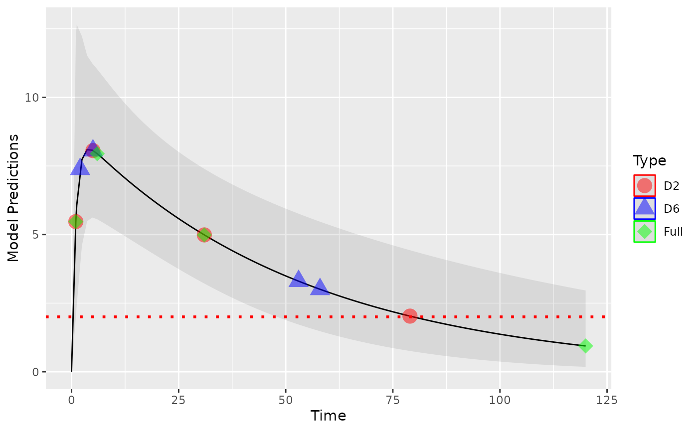
To compare the effects of these different designs on parameter precision, we evaluate each of the optimal designs above using the D6 method.
optim_full_D6<- with(optim_full,
  evaluate_design(poped.db,
                  loq=2))

optim_D2_D6<- with(optim_D2,
  evaluate_design(poped.db,
                  loq=2))

optim_D6_D6<- with(optim_D6,
  evaluate_design(poped.db,
                  loq=2))
The expected %RSE of the parameters is shown below. We see that the D6 optimized design gives, on average, the best parameter precision. The D2 optimal design stragetgy may be a reasonable obtain designs that are “good enough” if the D6 method is too slow for optimization.
optim_rse_D6 <-
  tibble::tibble("Parameter"=names(eval_full$rse),
                 "No LOQ"=round(optim_full_D6$rse),
                 "D6"=round(optim_D6_D6$rse),
                 "D2"=round(optim_D2_D6$rse))
optim_rse_D6| Parameter | No LOQ | D6 | D2 |
|---|---|---|---|
| CL | 7 | 5 | 6 |
| V | 4 | 3 | 3 |
| KA | 16 | 17 | 16 |
| d_CL | 67 | 34 | 43 |
| d_V | 58 | 54 | 52 |
| d_KA | 30 | 39 | 30 |
| sig_prop | 114 | 96 | 93 |
| sig_add | 152 | 60 | 92 |
References
Version information
sessionInfo()
#> R version 4.4.1 (2024-06-14)
#> Platform: x86_64-pc-linux-gnu
#> Running under: Ubuntu 22.04.5 LTS
#>
#> Matrix products: default
#> BLAS:   /usr/lib/x86_64-linux-gnu/openblas-pthread/libblas.so.3
#> LAPACK: /usr/lib/x86_64-linux-gnu/openblas-pthread/libopenblasp-r0.3.20.so;  LAPACK version 3.10.0
#>
#> locale:
#>  [1] LC_CTYPE=C.UTF-8       LC_NUMERIC=C           LC_TIME=C.UTF-8
#>  [4] LC_COLLATE=C.UTF-8     LC_MONETARY=C.UTF-8    LC_MESSAGES=C.UTF-8
#>  [7] LC_PAPER=C.UTF-8       LC_NAME=C              LC_ADDRESS=C
#> [10] LC_TELEPHONE=C         LC_MEASUREMENT=C.UTF-8 LC_IDENTIFICATION=C
#>
#> time zone: UTC
#> tzcode source: system (glibc)
#>
#> attached base packages:
#> [1] stats     graphics  grDevices utils     datasets  methods   base
#>
#> other attached packages:
#> [1] PopED_0.7.0      kableExtra_1.4.0 knitr_1.48       ggplot2_3.5.1
#>
#> loaded via a namespace (and not attached):
#>  [1] sass_0.4.9        utf8_1.2.4        generics_0.1.3    xml2_1.3.6
#>  [5] gtools_3.9.5      stringi_1.8.4     digest_0.6.37     magrittr_2.0.3
#>  [9] evaluate_1.0.0    grid_4.4.1        pkgload_1.4.0     mvtnorm_1.3-1
#> [13] fastmap_1.2.0     rprojroot_2.0.4   jsonlite_1.8.9    brio_1.1.5
#> [17] fansi_1.0.6       viridisLite_0.4.2 scales_1.3.0      codetools_0.2-20
#> [21] textshaping_0.4.0 jquerylib_0.1.4   cli_3.6.3         rlang_1.1.4
#> [25] munsell_0.5.1     withr_3.0.1       cachem_1.1.0      yaml_2.3.10
#> [29] tools_4.4.1       dplyr_1.1.4       colorspace_2.1-1  vctrs_0.6.5
#> [33] R6_2.5.1          lifecycle_1.0.4   stringr_1.5.1     fs_1.6.4
#> [37] htmlwidgets_1.6.4 ragg_1.3.3        pkgconfig_2.0.3   desc_1.4.3
#> [41] pkgdown_2.1.1     pillar_1.9.0      bslib_0.8.0       gtable_0.3.5
#> [45] glue_1.8.0        systemfonts_1.1.0 xfun_0.48         tibble_3.2.1
#> [49] tidyselect_1.2.1  highr_0.11        rstudioapi_0.16.0 farver_2.1.2
#> [53] htmltools_0.5.8.1 rmarkdown_2.28    svglite_2.1.3     labeling_0.4.3
#> [57] testthat_3.2.1.1  compiler_4.4.1